How to hide columns in Google Sheets

One of the major benefits of spreadsheets is that they can efficiently store and organize a lot of information — but working in a larger spreadsheet can be challenging. Google Sheets spreadsheets typically start out with 26 columns and 1,000 rows, meaning as you build out a spreadsheet, you can end up spending a lot of time scrolling through the information you’ve entered.

Hiding columns or rows can make a spreadsheet much more manageable. Whether you’re actively entering information in the sheet or want to be able to view and compare just a few columns at a time, this feature is a valuable tool that can make your life easier.

If you’re used to using Microsoft Excel, the “hide columns” feature in Google Sheets works slightly differently. This guide will take you through the steps.

How to hide a single column in Google Sheets

If you need to hide just one column, follow these steps:

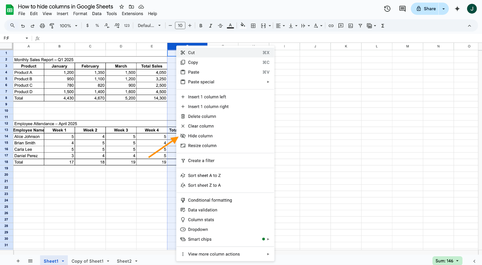
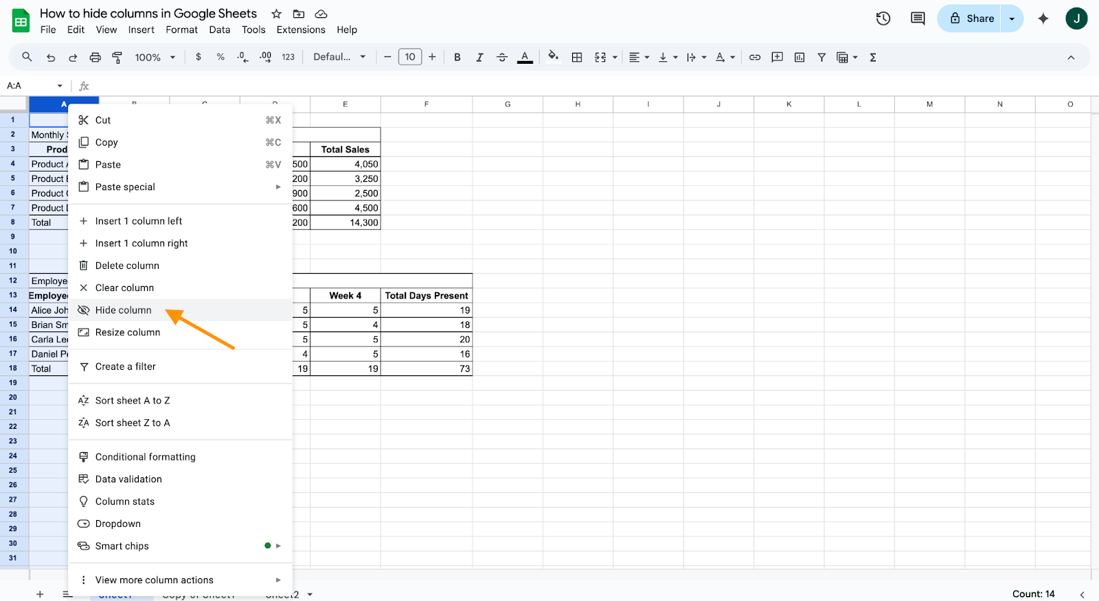
1. Right-click on the letter at the top of the column.
2. Choose Hide column from the dropdown menu.

You can hide a single row by right-clicking the number to the left of the row and choosing Hide row from the dropdown menu. 

How to hide multiple columns in Google Sheets

Sometimes you may need to hide multiple columns. While you can perform the above steps for each column separately, following the steps below will hide multiple columns (or rows) at once:

1. Click on a column header to select that column.
2. If you want to select columns that are contiguous to that first column, hold down the Shift key and click the headers of each additional column.
3. If you want to select columns that are non-contiguous to the first column, hold down the Control key (or the Command key on a Mac) as you click each column header.
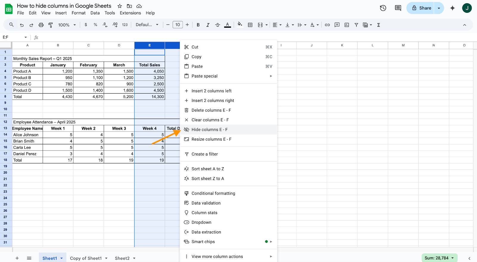
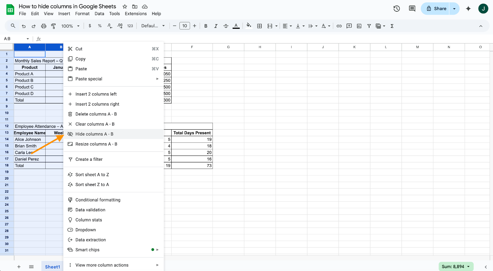
4. Once you’ve selected all of the columns you want, right-click within one of the selected columns.
5. Choose Hide columns X–X from the dropdown menu. (“X–X” represents the range of column letters you’re hiding.)

This process also works to hide rows.

How to hide columns in Google Sheets using keyboard shortcuts

To hide a column using a keyboard shortcut, first click on the column header and then use the following shortcut:

• Control + ALT + 0
• Command + Option + 0 (on a Mac)

This shortcut will hide the column(s) you’ve selected. Alternatively, you can just click in a cell within the column and then use the shortcut; it will still hide the column.

How to hide unused columns

Unused columns can be distracting, but you can easily hide them to help you focus only on the active areas of your sheet.

1. Click on the column header of the first column that appears to the right of the last column you’re using in the sheet. In other words, highlight the first column that you want to hide.
2. Hold down the Control and Shift keys simultaneously (or the Command and Shift keys on a Mac). While you’re holding down these keys, press the right arrow key. All of the unused columns should now be selected.
3. Right click on any selected column to open the dropdown menu.
4. Select the Hide columns X–X option. (Again, the “X–X” should reflect the names of the range of selected columns.)

How to hide columns or rows on Android or iOS

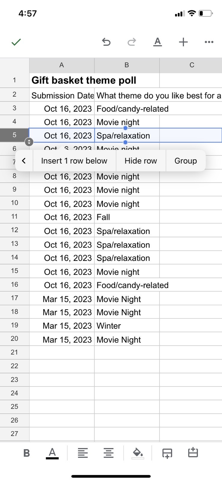
You can also easily hide rows in Google Sheets on your Android or iOS mobile phone. Here’s how.

1. Open the Google Sheets app.
2. Open a Google Sheet.
3. When using an iPhone, select the rows that you want to hide, then tap on those rows. A menu will appear; tap Hide row.

4. When using an Android phone, tap and hold the row that you want to hide. A menu will appear above the row. Tap on the three vertical dots, then tap on Hide row.

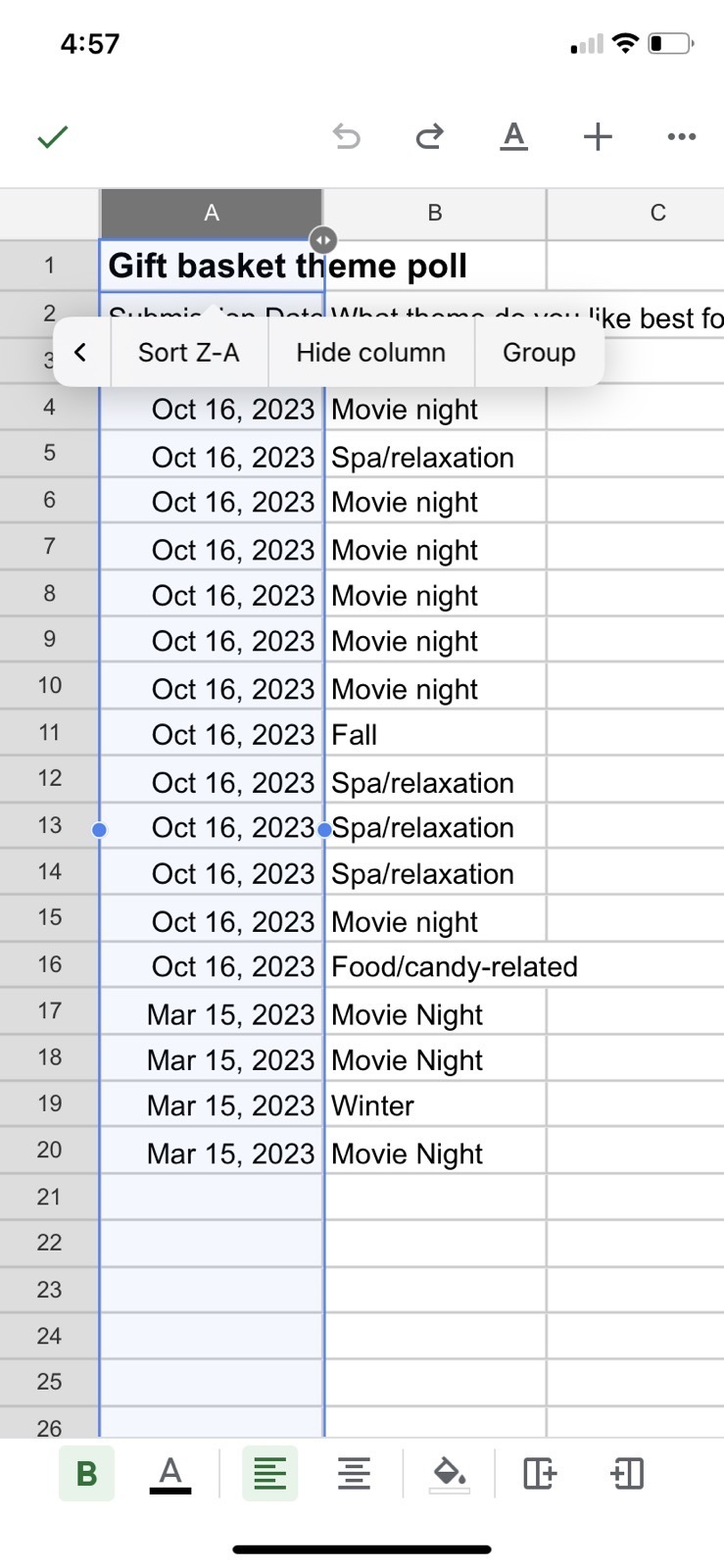
The process is similar if you want to hide columns using your phone:

1. Open the Google Sheets app.
2. Open a Google Sheet.
3. When using an iPhone, select the columns that you want to hide, then tap on those columns. A menu will appear; tap Hide column.

4. When using an Android phone, tap and hold the column that you need to hide. A menu will appear above the column. Tap on the three vertical dots, then tap Hide column.

How to unhide columns in Google Sheets

When you need to see or work within the columns that you’ve hidden, you can easily unhide them.

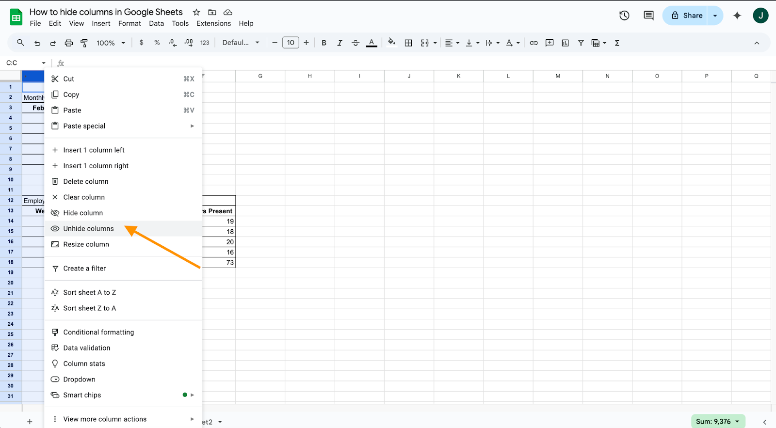
1. To find your hidden columns, look at the column headings. You’ll see small arrows pointed away from each other positioned in some column headings. These arrows identify areas where columns are hidden.
2. Click on the arrow icon to unhide all of the columns that are hidden in that location.

Putting the power of Google Sheets to work for your business

Google Sheets is a powerful tool, and it gives you and your team the ability to easily and effectively collaborate on everything from budgets to campaign plans and more. To maximize the effectiveness of Google Sheets, take some time to learn the basic functions — like how to lock cells, wrap text, and sort data.

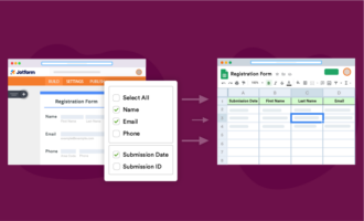
There are plenty of other ways to put Google Sheets to work for your business, though. Google Sheets integrates with several data-collection tools, including Jotform. 

You can save time by integrating Jotform with Google Sheets to get real-time updates of your data as users fill out forms. You can also use Google Sheets to create Gantt charts, to-do lists, monthly budgets, and more. Jotform table templates can also help you perform these types of tasks.

The more you use Google Sheets, the more you’ll learn about its functionality and the different ways you can put it to use for your business. This powerful program allows for seamless collaboration across your business teams. And its functionality resembles what you get with Microsoft Excel, so it’s a great option for businesses of all sizes.